Sixth Edition | January 2024
RESOURCES: read report as PDF | view state profiles | use data visualizations | download full dataset
EXECUTIVE SUMMARY
In the United States, K-12 school finance is largely controlled by the states. Every year, hundreds of billions of dollars in public funds are distributed based on 51 different configurations of formulas, rules, and regulations to over 13,000 districts that vary in terms of the students they serve, their ability to raise revenue locally, and many other characteristics.
In this sixth edition of our annual report, we evaluate the K-12 school finance systems of all 50 states and the District of Columbia. The latest year of data we present is the 2020-21 school year.
Good school finance systems compensate for factors states cannot control (e.g., student poverty, labor costs) using levers that they can control (e.g., driving funding to districts that need it most). We have devised a framework that evaluates states based largely on how well they accomplish this balance. We assess each state’s funding while accounting directly for the students and communities served by its public schools.
This is important because how much a given district or state spends on its schools, by itself, is a rather blunt measure of how well those schools are funded. For example, high-poverty districts require more resources to achieve a given outcome goal—e.g., a particular average score on a standardized test—than do more affluent districts. In other words, education costs vary depending on student populations, labor markets, and other factors. That is a fundamental principle of school finance. Simply comparing how much states or districts spend ignores this enormous variation in how much they must spend to meet their students’ needs.
The key question, then, is not just how much states and districts spend but whether it’s enough—is funding adequate for students from all backgrounds to achieve common outcome goals?
Accordingly, we use a national cost model to calculate adequate funding levels for the vast majority of the nation’s public school districts. We then use these estimates to evaluate each state—relative to other states or groups of states—based on the overall adequacy of funding across all its districts (statewide adequacy) as well as the degree to which its high-poverty districts are more or less adequately funded than its affluent districts (equal opportunity). Finally, because states vary in their ability to raise revenue (e.g., some states have larger economies than others), we also assess whether states are leveraging their capacity to fund schools by measuring total state and local spending as a percentage of states’ economies (fiscal effort).
These three “core indicators”—effort, statewide adequacy, and equal opportunity—offer a parsimonious overview of whether states’ systems are accomplishing their primary goal of providing adequate and equitable funding for all students. In this report, as well as the one-page state profiles that accompany the report, we present results on these three measures for each state.
Selected national findings
There are 39 states that devote a smaller share of their economies to their K-12 schools than they did before the 2007-09 recession. This cost schools over $360 billion between 2016 and 2021, which is 9 percent of all state and local school funding during those six years.
- This includes several states with enormous proportional “losses” between 2016-2021, such as Hawaii (-27.8 percent), Arizona (-27.5 percent), Indiana (-26.8 percent), Florida (-24.9 percent), Michigan (-20.0 percent), and Idaho (-19.9 percent).
- In other words, had these states recovered to their own 2006 effort levels by 2016, their total state and local school funding between 2016 and 2021 would have been 20-28 percent higher.
About 60 percent of the nation’s students that we identify as being in “chronically underfunded” districts—the 20 percent of districts with the most inadequate funding in the nation—are in just 10 states. These states (Alabama, Arkansas, Florida, Georgia, Louisiana, Mississippi, Nevada, New Mexico, North Carolina, and Texas) serve only about 30 percent of the nation’s students.
- Three of these states (Florida, Nevada, and North Carolina) are comparatively low fiscal effort states, which suggests they have the capacity to increase funding substantially but are not doing so.
- In contrast, three of them (Arkansas, Mississippi, and New Mexico) are high effort states, but their economies are so small—and their costs so high—that they would have trouble providing adequate funding even at much higher effort levels. We argue that these states are most in need of additional federal aid.
African American students are twice as likely as white students to be in districts with funding below estimated adequate levels, and 3.5 times more likely to be in “chronically underfunded” districts. The discrepancies between Hispanic and white students are moderately smaller but still large.
Educational opportunity is unequal in every state—that is, higher-poverty districts are funded less adequately than lower-poverty districts. But the size of these “opportunity gaps” varies widely between states.
- The largest gaps (most unequal opportunity) tend to be in states, such as Connecticut, New York, and Massachusetts, where statewide adequacy is relatively high, but where wealthier districts contribute copious amounts of local (property tax) revenue to their schools. This exacerbates the discrepancies in funding adequacy between these districts and their less affluent counterparts.
- States should narrow these adequacy gaps by targeting additional state aid at higher-poverty districts with less capacity to raise revenue locally.
Policy recommendations
Based on the results of this report, we conclude with a set of basic, research-backed principles that should guide the design and improvement of all states’ systems.
Better targeting of funding. If district funding levels are not determined rigorously by states, resources may appear adequate and equitable when they are not (and policymakers may not even realize it). All states should routinely “audit” their systems by commissioning studies to ensure that they are accounting for differences in the needs of the students served by each of their school districts.
Increase funding to meet student needs where such funding is inadequate. The point here is for states to ensure that funding is commensurate with costs/need. In some states, adequate and equitable funding might require only a relatively modest increase in total funding (particularly state aid) along with better targeting. In other states, particularly those in which funding is inadequate and effort is low, larger increases are needed, and may include both local and state revenue.
Distribute federal K-12 aid based on both need and effort. The unfortunate truth is that many states with inadequate funding put forth strong effort levels but do not have the economic capacity to meet their students’ needs. For these states, additional federal education aid can serve as a vital bridge to more adequate and equitable funding.
Enhance federal monitoring of school funding adequacy, equity, and efficiency. We propose that the U.S. Department of Education establish a national effort to analyze the adequacy and equity of states’ systems and provide guidance to states as to how they might improve the performance of those systems.
Our findings as a whole highlight the enormous heterogeneity of school funding, both within and between states. Such diversity is no accident. So long as school finance is primarily in the hands of states, the structure and performance of systems is likely to vary substantially between those states.
The upside of this heterogeneity is that it has allowed researchers to study how different systems produce different outcomes and, as a result, we generally know what a good system looks like. Our framework for evaluating states is based on these principles. It is our hope that the data presented in this report and accompanying resources will inform school finance debates in the U.S. and help to guide legislators toward improving their states’ systems.
Continue reading full report below or download report as PDF
HOW WE EVALUATE STATES’ K-12 FINANCE SYSTEMS
A state school finance system is a collection of rules and policies governing the allocation of state and local K-12 school funding. On average, about 90 percent of school funding comes from a combination of local and state revenues, with the remainder coming in the form of federal aid. Many states’ systems are exceedingly complicated, with numerous formulas, rules, and regulations that have evolved over decades of political wrangling, advocacy, and litigation. Yet all systems can be described—and evaluated—in terms of the following two goals:
- Account for differences in the costs of achieving equal educational opportunity across school districts. Proper determination of districts’ costs—setting “funding targets” for each district, whether implicitly or explicitly—is the foundation of any state’s system. If that is done poorly, then the entire funding process may be compromised. Cost refers to the amount of money a school district needs to meet a certain educational goal, such as a particular average score on a standardized test or a graduation rate. Costs vary within states because student populations vary (e.g., some districts serve larger shares of disadvantaged students than others) and also because the economic and social characteristics of school districts vary (e.g., some districts are located in labor markets with higher costs of living than others). School funding formulas should attempt to account for these differences by driving additional state aid to districts with higher costs.
- Account for differences in fiscal capacity, or the ability of local public school districts to pay for the cost of educating their students. Although the extent varies, school districts in all states rely heavily on local revenue (mostly from property taxes) to fund schools. Wealthier communities, of course, can raise more and tax themselves at lower rates. School funding formulas attempt to compensate by directing more state aid to districts with less capacity to raise local revenues.
Whether or not states accomplish these goals carries serious consequences for millions of public school students. Over the past 10-15 years, there has emerged a growing consensus, supported by high-quality empirical research, that additional funding improves student outcomes and that funding cuts hurt those outcomes, particularly among disadvantaged students (Baker 2017, 2018; Candelaria and Shores 2019; Handel and Hanushek 2023; Jackson 2020; Jackson, Johnson, and Persico 2016; Jackson, Wigger, and Xiong 2021; Jackson and Mackevicius 2023; Lafortune, Rothstein, and Schanzenbach 2018).
There are, of course, important debates about how education dollars should be spent. Yet schools cannot spend money they do not have, and proper funding is one necessary requirement for improving student outcomes. Understanding, assessing, and reforming states’ funding systems is therefore a crucial part of any efforts to bring about such improvement.
Evaluation framework
Our framework for evaluating the K-12 finance systems of all 50 states and the District of Columbia begins with two basic premises, both discussed above:
1a. Higher student outcomes require more resources; and
1b. The cost of achieving a given outcome varies by context.
The importance of context (1b) is critical to understanding and measuring costs, and thus to our approach to evaluating states’ systems. By context, we mean not only the population a district serves (e.g., poverty), but also the labor market in which it is located, its size (economies of scale), and other factors that can affect the “value of the education dollar.” Any serious attempt to compare funding between states—or between districts within a given state—must address the fundamental reality that the “cost of education” is far from uniform.
Consider, for example, two hypothetical school districts, both of which spend the same amount per pupil. The simple approach to comparing these two districts might conclude that they invest equally in resources, such as teachers, curricular materials, etc., that can improve student performance.
If, however, one of these districts is located in an area where employees must be paid more due to a much more competitive labor market or higher cost of living, or if it serves a larger proportion of students with special needs, then this district will have to spend more per pupil than its counterpart to provide a given level of education quality (i.e., to achieve a common student outcome goal or goals). Controlling for these factors does not, of course, guarantee accuracy or comparability, but failure to do so is virtually certain to lead to misleading conclusions.
It follows directly from these first two tenets (1a and 1b) that the key question in evaluating finance systems is not just how much states or districts spend but, perhaps more important, whether it is enough—i.e., whether resources are adequate to meet costs (note that we use the terms “costs,” “adequate funding levels,” and “funding targets” interchangeably).
Our second set of principles pertains to how we define this key concept of adequacy. Since the core purpose of public schools is to educate and prepare all students:
2a. We define adequacy as the cost of achieving student outcome goals; and
2b. We estimate costs in all states and districts with reference to the same outcome goals—that is, when evaluating the performance of states’ systems, the adequacy of funding should not be judged using a high “benchmark” goal in some states and a more modest goal in other states.
Regarding 2b, we recognize that states vary in terms of their academic standards and/or in the outcome goals that their finance systems are (at least in theory) calibrated to produce. Our purpose, however, is to evaluate all states’ systems in a comparable manner, and doing so requires common outcome goals within and between states. This means that estimated adequate spending levels will vary by district (see 1b), but those levels represent the cost of achieving the same benchmark goals.
Our third principle is methodological, but it is worth stating directly:
.
3. The most appropriate approach to a national evaluation of K-12 funding adequacy, which requires the estimation of costs across thousands of heterogeneous districts serving millions of diverse students, is to use statistical cost models (education cost functions).
.
There are a variety of different approaches that researchers use to estimate costs (or that states use to determine district funding targets). The options include everything from sophisticated statistical models to more ad hoc costing studies and formulas to “professional judgment panels” of experts. We use cost modeling, and we argue it’s the best option in the context of a national analysis of states’ systems.[1] We describe our model in more detail in the next section.
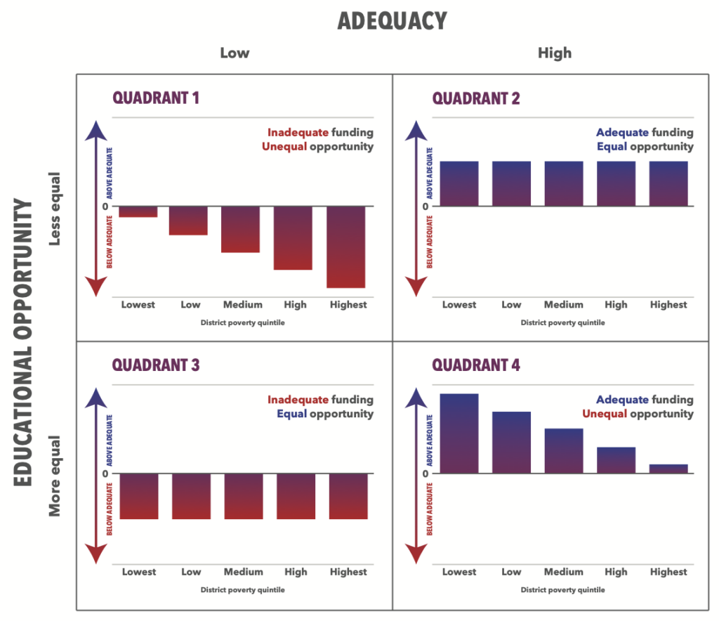
Insofar as the primary goal of any state finance system is to provide all students with an equal shot at achieving common outcomes, we use our cost model estimates to evaluate states on two adequacy-focused dimensions or measures (statewide adequacy and equal opportunity), which represent two of our three “core indicators.” They are the degree to which states:
.
4a. Provide all students with enough funding to achieve a common outcome goal (i.e., statewide adequacy); and
4b. Ensure that no students have a greater chance of achieving those goals than do their peers elsewhere in the state (i.e., equal opportunity).
.
It is important to note that these two indicators—statewide adequacy and equal opportunity—are conceptually independent. That is, one can exist without the other. There may, for example, be states in which relatively large proportions of students attend districts with funding above estimated adequate levels (i.e., high statewide adequacy), but in which funding is far above adequate levels in some districts and just barely above in others (unequal opportunity). Conversely, states can exhibit comparatively low adequacy, with wide swaths of underfunded districts, but still maintain equal opportunity, if all districts are generally the same “distance” away from (in this case, below) their estimated adequate funding levels.
States’ systems should ideally provide both adequate funding and equal opportunity—i.e., funding in all districts is either at adequate levels or above those levels by roughly the same proportional amount.[2] But states can be evaluated on each dimension separately.
The final element of our framework for evaluating states’ K-12 finance systems is designed to account for the aforementioned fact that both costs and the ability to raise revenue to pay those costs differ between states. Our fifth principle, therefore, is the basis for our third and final core indicator (fiscal effort), and it is:
5. States should also be evaluated on how much of their economic capacity—i.e., their ability to raise revenue—is devoted to their public schools (i.e., fiscal effort).
Some states’ economies are so small relative to their students’ needs that they are essentially unable to raise enough revenue to fund their schools adequately, whereas other states simply fail to provide sufficient resources despite having the option to do so. Including effort in our framework allows us to differentiate the former states from the latter.
Our adequacy estimates
Our adequacy estimates play a central role in our system—i.e., they are used directly in calculating two of our three core indicators (statewide adequacy and equal opportunity). The cost model from which these estimates are derived is called the National Education Cost Model, or NECM. The NECM is part of the School Finance Indicators Database (SFID), which is a set of public data and resources on state and local school finance that we update and publish annually, and from which all the measures presented in this report are drawn.
The NECM estimates how much each district must spend (i.e., costs) to achieve a common benchmark outcome goal. We choose to set this goal as national average math and reading scores in grades 3-8. This is a relatively modest goal, but we interpret our adequacy results such that choosing a different benchmark would not substantially alter our conclusions about the performance of states’ systems.[3]
This model yields these estimated adequate funding levels every year for over 12,000 districts, which serve about 95 percent of the nation’s students. The estimates are based on numerous factors, including each district’s Census child poverty rate, its labor costs (if the cost of living in a district is higher it must pay its employees more), its size (economies of scale), its students’ characteristics, and other factors.[4] We then compare those estimated adequate funding levels to actual funding (spending) levels.
A problem with cost modeling in education finance is that outcomes and spending have a circular, or endogenous,relationship. Greater spending leads to better educational outcomes; however, better outcomes can lead to greater spending, as higher test scores can manifest in higher property values, increasing a community’s tax capacity and, therefore, its ability to spend on its schools (Figlio and Lucas 2004; Nguyen-Hoang and Yinger 2011). The NECM draws on previous work in education cost modeling to address this problem through econometric methods (for more technical details on the model, see Baker, Weber, and Srikanth [2021]).
It’s important to bear in mind the limitations of our adequacy measures. Like any tools for assessing finance systems, they are imperfect. There is the normal, inevitable imprecision of any complex statistical model (which is an issue regardless of approach, of course), including the fact that we cannot control for absolutely everything that affects costs (researchers call this “omitted variable bias”).
But there is also an additional layer of imprecision when you’re looking at all states simultaneously. There are, for example, inconsistencies between states in how they collect finance data and report it to the U.S. Census Bureau. Similarly, we are relying on an outcome dataset (the Stanford Education Data Archive) that transforms the results of all states’ standardized tests such that they can be compared across the nation (Reardon et al. 2021); these data, though groundbreaking, may also contain inconsistencies due to the normalization process. In part for these reasons, one of our recommendations, discussed below, is for states to commission their own cost model studies, using their own state-specific testing and finance data.[5]
And, finally, there is one additional consideration here, which affects the interpretation of adequacy estimates (or any funding measures) in any context: cost models are essentially designed to isolate the (bi-directional) effect of spending on testing outcomes, but some districts are more efficient than others in how they spend money. So, for instance, what seems like inadequate funding might be due in part to inefficiency. Similarly, many districts, particularly affluent districts, spend money on programs or facilities that don’t necessarily affect standardized math and reading test scores but may still be highly desirable to students and parents.
All that said, we contend that our adequacy (NECM) estimates, interpreted properly, are superior to the alternatives (and, if we’re talking about national cost estimates based on inputs and student outcome goals, the NECM, to our knowledge, is the only option). They are not designed to be interpreted as purecausal estimates in the sense that we can say “if you spend X number of dollars you will achieve Y level of test scores.” Even if we had a way to calculate perfect estimates of education costs, we would not imply that these spending levels, if put into place in a state or district, would quickly and certainly raise scores to the national average. This is not only because that implication assumes efficient use of additional funds, but also because real improvement is gradual and requires sustained investment.
Our model, rather, yields reasonable estimates of costs that allow for better evaluations of states’ finance systems toward the goal of improving those systems. Yet we are mindful of their limitations, and so we try to be careful and clear about how we use them to evaluate states’ systems. There are two general purposes:
- Comparisons between states: We average our district estimates across entire states and use them to compare statewide adequacy and equal opportunity (see below) between those states.
- Comparisons within states (or over time): This is very similar to the between-state comparisons, except instead of averaging our district estimates across a whole state, we average and compare them within states (e.g., by district poverty, student race/ethnicity, or over time).
The key point here is that we are interpreting each state’s results relatively. We generally avoid, for example, using our estimates to state with confidence whether a state’s schools are funded adequately by some absolute standard. We do, however, say—with due caution—whether that state’s schools are more or less adequately funded than those in a different state or group of states, or whether different groups of districts are funded more or less adequately than others within a state.
The COVID-19 pandemic and school funding
The COVID-19 pandemic did not cause the catastrophic budget cuts that many were anticipating in mid-2020 (Baker and Di Carlo 2020). This was due in large part to the relatively quick recovery of most states’ economies, and certainly the K-12 fiscal situation was also shored up by the roughly $200 billion in federal pandemic aid to schools allocated in three waves under the banner of the Elementary and Secondary School Emergency Relief (ESSER) Fund. Much recent debate about school finance has focused on concerns about what will happen when this money stops flowing to districts over the next couple of years. This will be a very important issue for schools and districts, but its implications for our measures are likely much less severe.
For instance, regarding this year’s results, the latest year of data presented in this report is 2021 (the 2020-21 school year), and our adequacy measures focus on spending, which includes federal (and, thus, ESSER) aid. However, only a relatively small share of these funds were being spent during the 2020-21 school year. This will increase in subsequent releases of our data.
Yet we do not anticipate that these additional federal funds, even when they do appear in our data, will have a large impact on our statewide adequacy and equal opportunity results (and none in the case of fiscal effort, which includes only state and local funding). Although the overall amount of this aid is large, the funding is spread out over multiple years and in most cases will not amount to a large proportional increase at the district level in any given year (especially when averaged across states). And, of course, any discernible impact will be temporary, as the additional ESSER funds will run out. Finally, and most importantly, we interpret our results relatively (e.g., by comparing states with each other in any given year). While the infusion of ESSER funds may affect our statewide adequacy and especially our equal opportunity results in absolute terms (e.g., funding may be more adequate, or less inadequate, in districts that receive the money), its impact on states’ relative performance will be less pronounced. Yet it is certainly something that we will be monitoring in future releases.
That said, recent national testing data suggest that the pandemic had a rather severe negative impact on the testing performance of the current cohort of U.S. students, particularly disadvantaged and struggling (lower-scoring) students (National Center for Education Statistics 2022). We would suggest that one major reason why students in higher-poverty districts bore the brunt of the ill effects—as well as why they were so far behind even before the pandemic—is the vast differences in the adequacy of resources between these districts and their more affluent counterparts. In addition, we contend that gaining back some of the ground these students have lost due to the pandemic’s disruption of in-person schooling will require fundamental changes in the levels and distribution of K-12 funding.
RESULTS
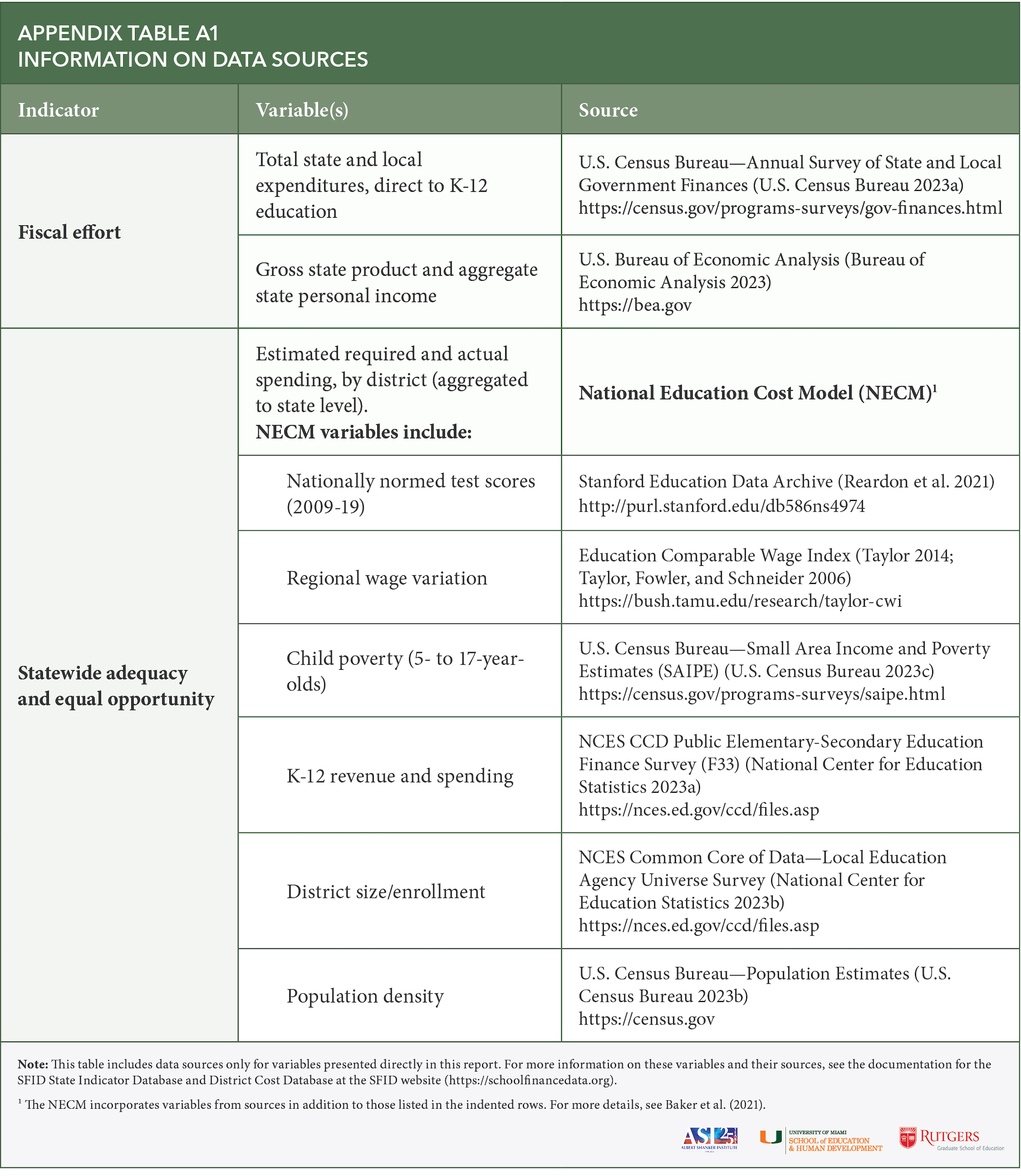
In this section, we report results for our three core indicators of fiscal effort, statewide adequacy, and equal opportunity. We then present overall scores for each state’s system based on their performance on these three indicators. Data sources for all measures are presented in Appendix Table A1.
Note that, throughout this report, individual years refer to the spring semester of that school year. For example, 2021 means that the data pertain to the 2020-21 school year (the most recent year available).
FISCAL EFFORT
Fiscal effort (or simply “effort”) measures how much of a state’s total resources are spent directly on K-12 education. In our system, effort is calculated by dividing total expenditures (state plus local, direct to K-12 education) by gross state product (GSP).[6] To reiterate, the effort numerator (total state and local spending) does not include federal aid; effort is strictly a state and local measure.
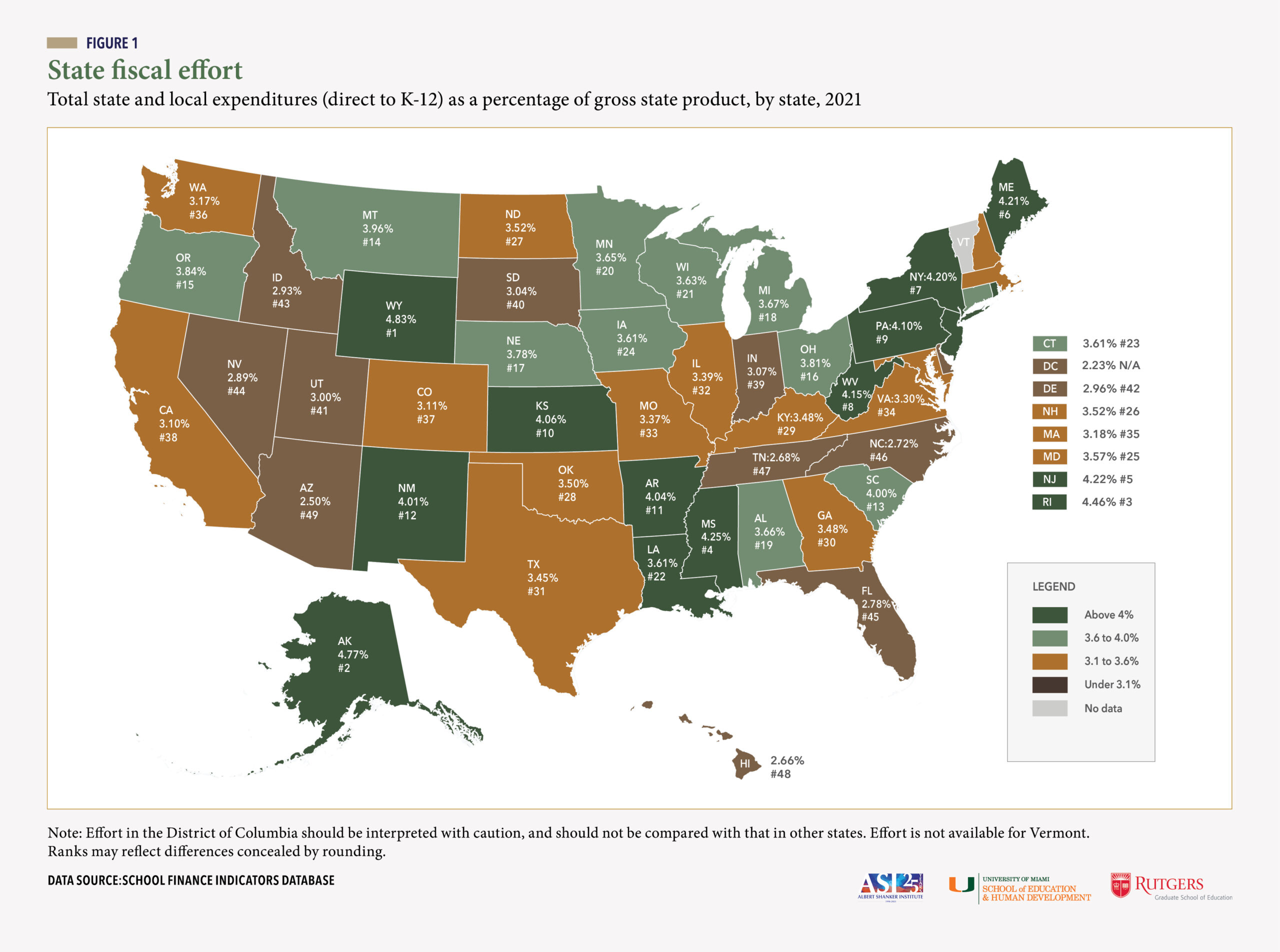
In Figure 1, we present a map with each state’s effort level in 2021, along with its rank (note that effort in the District of Columbia is reported in Figure 1 but it should not be compared with that in other states). Effort ranges from approximately 2.5 percent in Arizona to around 4.8 percent in Alaska and Wyoming. Put differently, if Arizona were to increase its effort level to that of Alaska and Wyoming, K-12 funding in Arizona would increase about 90 percent.
In addition to Alaska and Wyoming, other particularly high effort states include Rhode Island (4.46 percent), Mississippi (4.25), New Jersey (4.22), and Maine (4.21). In contrast, the states in which spending as a proportion of capacity is lowest (other than the District of Columbia, which, again, should not be compared with other states) are Arizona (2.50 percent), Hawaii (2.66), Tennessee (2.68), North Carolina (2.72), and Florida (2.78).
Most states are clustered within 0.5 percentage points of the unweighted U.S. average of 3.53 percent. But even seemingly small differences in effort represent large amounts of school funding. As an illustration, in the typical state, a 0.5 percentage point (one-half of 1 percentage point) increase in effort would be equivalent to roughly a 15 percent increase in K-12 funding. We shall return to these state-by-state effort results when we discuss statewide adequacy, below.
Fiscal effort trend 2006-2021
States’ fiscal effort levels can vary year to year due to changes in their education funding policies, their overall economies (e.g., GSP), or both. Figure 2 presents the national trend in effort between 2006 and 2021. The figures in the graph are unweighted averages—i.e., each state’s effort level counts equally toward the national average in any given year. They provide a sense of changes over time in how much the typical state is spending as a share of its capacity.
Fiscal effort seems quite volatile during the earlier years of this time period. The primary reason for this is the financial crisis and so-called Great Recession of 2007-09. Effort spiked between 2007 and 2009 and subsequently declined sharply between 2009 and 2013. The initial jump (2007-09) is an “illusion” of sorts, a result of the fact that recessions affect the denominator of the effort equation (capacity, or GSP) before they affect the numerator (spending). Recessions cause economies to contract very rapidly (they are of course defined that way). But school budget cuts usually take longer to appear. As a result, education spending (the numerator) in the typical state was relatively stable for a couple of years (2007-2009) while capacity (the denominator) declined, causing a spike in effort even without an unusual increase in K-12 spending.
The situation changed dramatically around 2009, as states’ economies began to recover while state and local budget cuts began to take effect. Average effort decreased sharply (almost 0.5 points) between 2009 and 2013, with at least a nominal net decrease during this time in every state except Delaware and Wyoming (where it was essentially unchanged) and the District of Columbia. This is a massive drop in U.S. average effort over a relatively short period of time, and, as we’ll see, it represents the loss of billions of dollars in education resources.
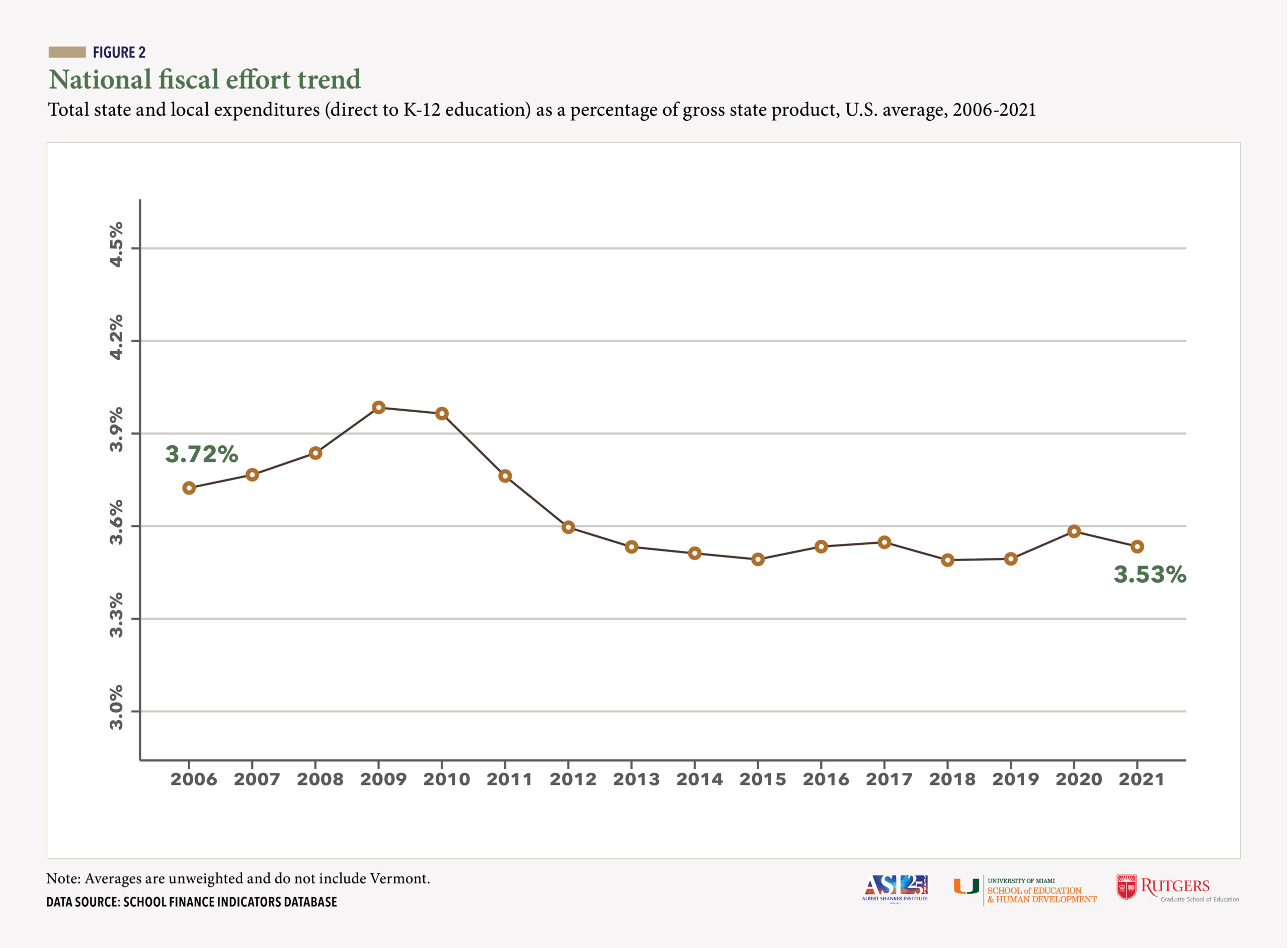
To reiterate, economic downturns tend to create these up-and-down periods, and the severity of the 2007-09 recession meant that this pattern was also going to be unusually pronounced. What’s truly disturbing—and unusual—is the fact that effort never recovered. Between 2013 and 2021, when our data end, effort in the typical state remained mostly flat, except for a jump between 2019 and 2020. Even this increase, however, was likely also an “illusion”—much like that which occurred between 2007 and 2009, except far less pronounced—and it does not reflect a concurrent increase in educational investment. During the first two quarters of 2020, the COVID-19 pandemic caused rather severe contractions of states’ economies (due to unemployment, shuttering and closing of businesses, etc.). This decrease in the effort denominator, along with comparatively flat state and local education spending, generated at least a nominal increase in effort in all but five states. In Figure 2 we can already see effort going back down to its pre-pandemic levels between 2020 and our most recent year of 2021. Whether it has declined below its pre-pandemic levels remains to be seen.
Even with this (likely temporary) net increase between 2019 and 2021, the U.S. average effort level was still lower in 2021 than at any point in nearly a decade, and 2021 effort was higher than it was in 2006 in only 11 states, typically by modest margins. In some states, the declines are alarming. The net decrease between 2006 and 2021 was greater than 0.5 percentage points (one-half of 1 percentage point) in ten states: New Jersey (-1.01 percentage points); Florida (-0.79); Indiana (-0.78); Idaho (-0.77); Arizona (-0.76); South Carolina (-0.64); Michigan (-0.63); Hawaii (-0.62); California (-0.54); and West Virginia (-0.54). To view the full trends for any state, download its one-page profile.
These trends since the 2007-09 recession are in no small part the result of deliberate choices on the part of policymakers in many states to address their recession-induced revenue shortfalls primarily with budget cuts rather than a mix of cuts and revenue-raising. In fact, a number of states actually cut taxes during and after the recession (Leachman, Masterson, and Figueroa 2017).
The cost of declining fiscal effort
The implications of what seems to be a permanent decline in most states’ K-12 effort levels are difficult to overstate. The changes in U.S. average effort discussed above may appear small—fractions of 1 percent—but, to reiterate, they can represent very large increases or decreases in education resources. The denominators of the effort calculation are entire state economies.
One simple way to illustrate this impact is to “simulate” spending in recent years at states’ pre-recession effort levels. For instance, we might ask: How much higher would total K-12 state and local spending have been between 2016 and 2021 had all states recovered to their own pre-recession (2006) effort levels by 2016? This “thought experiment” entails simply multiplying each state’s 2006 effort level by its gross state product in each year between 2016 and 2021 and comparing those amounts with actual total state and local spending.
According to these calculations, the failure of states to make their districts whole after the 2007-09 recession cost public schools a total of roughly $364 billion between 2016 and 2021, which is about 9 percent of all state and local funding over these six years. And this includes enormous proportional “losses” in Hawaii (-27.8 percent), Arizona (-27.5), Indiana (-26.8), Florida (-24.9), Michigan (-20.0 percent), and Idaho (-19.9 percent). In other words, had these states recovered to their own 2006 effort levels by 2016, their school funding between 2016 and 2021 would have been 20-28 percent higher than it was.
Seven states, to their credit, had higher effort levels in all six years than they did in 2006: Alaska; Connecticut; the District of Columbia; Louisiana; Minnesota; Nebraska; and Wyoming. Three additional states—Oregon, Rhode Island, and Washington—saw minimal “losses” (less than 0.1 percent). To view the results of this simulation for a state not mentioned above, download that state’s one-page profile.
STATEWIDE ADEQUACY
As discussed above, our adequacy measures compare actual spending per pupil to estimated (cost-modeled) per-pupil spending levels that would be required to achieve the common goal of national average math and reading test scores. We call these latter estimates “costs,” “estimated adequate funding levels,” and “funding targets” interchangeably.
There are different ways to express statewide adequacy. The most “direct” statistic might be the (enrollment-weighted) average percentage difference between actual spending and estimated adequate spending (i.e., each state’s “adequate funding gap”). These estimates are presented in Appendix Table A2. If, for example, a state’s adequate funding gap is -15 percent, that means the typical student’s school district in that state spends 15 percent below our estimated adequate funding levels.
In this section, we focus instead on a measure that is very highly correlated with the adequate funding gaps but is somewhat simpler and more intuitive: the percentage of students in each state who attend schools in districts where actual spending is below estimated adequate spending.
We also identify a subset of these below adequate districts in which spending is particularly far below adequate levels. We refer to these as “chronically below adequate”—or “chronically underfunded”—districts. We identify these districts as the 20 percent of all U.S. districts with the largest negative adequate funding gaps as a percentage (i.e., the 20 percent of all districts in which actual spending is furthest below estimated adequate spending). We then calculate, just as above, the proportion of each state’s students attending one of these districts. The purpose of looking at the percentage of students in both below adequate and chronically below adequate districts is that the latter statistic gives a sense of how many students in each state are in districts where funding is so low relative to costs that additional funding is especially urgent.
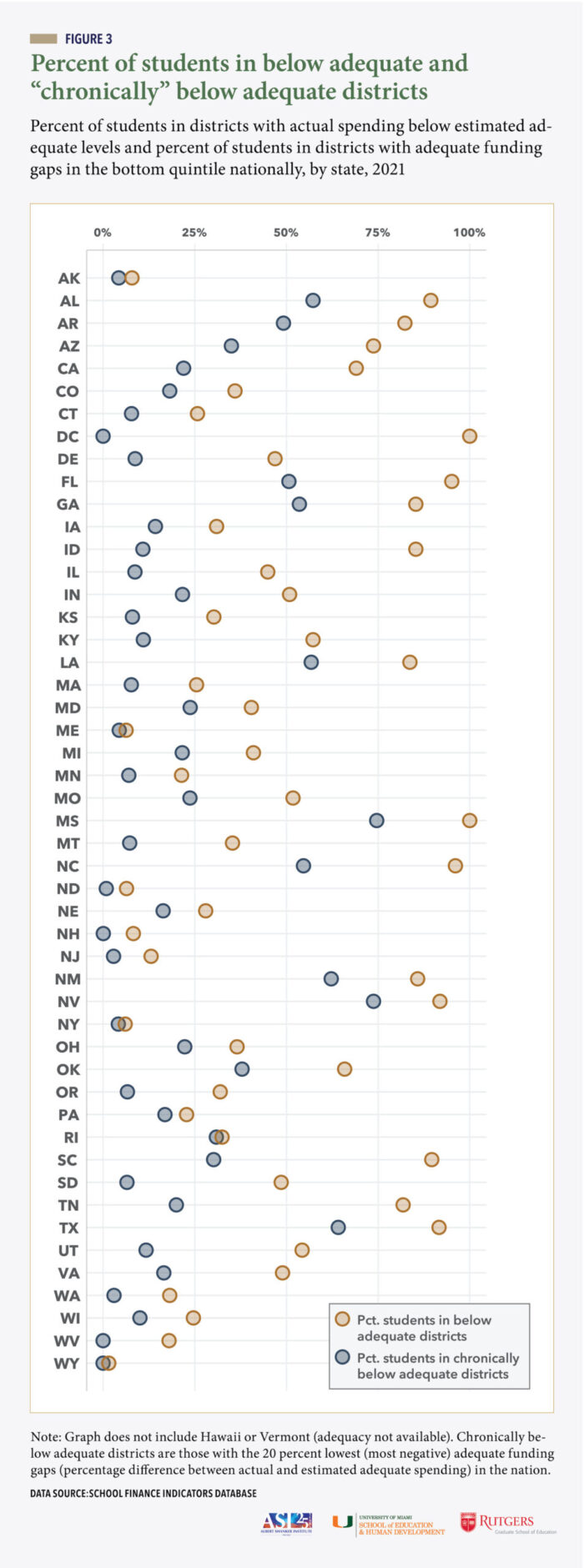
In Figure 3, we present the percentage of students in each state in below adequate (tan circles) and chronically below adequate districts (blue circles).[7] Obviously, circles further to the left indicate more adequate funding (i.e., lower proportions of students in districts with below adequate funding). We would reiterate that it is best to interpret the percentage in each state relative to those in other states. For example, in Maine, only about 6 percent of students attend schools in below adequate districts, and just over 4 percent are in chronically underfunded districts. We cannot say, for the reasons discussed above, that these are the “true” percentages, but we would conclude that Maine districts, on average, are among the most adequately funded in the nation (the circles in Figure 3 are further to the left than they are in most other states). Relatively low proportions of students are in below adequate districts in several other states, including Wyoming (1.5 percent), New York (6.0), North Dakota (6.4), Alaska (7.8), and New Hampshire (8.2).
Mississippi, in contrast, has the highest percentages of students in both underfunded and chronically underfunded districts (100 and 75 percent, respectively). Yet Mississippi also devotes a relatively large share of its economy to its schools—i.e., it puts forth relatively high effort (see Figure 1). And this same basic finding—relatively low adequacy, relatively high effort levels—also applies to other states, such as Arkansas, New Mexico, and South Carolina.
This, to reiterate, is in part because students in these states are especially higher in poverty compared with students in other states, and their students tend to score relatively low on state tests. As a result, these states have higher costs, and must spend more to achieve a common student outcome goal, making adequacy more difficult even if effort is high. But it is also because of the (related) fact that these are comparatively low-capacity states. That is, due to their small economies, their high effort levels still generate less revenue than those effort levels would yield in states with larger economies (e.g., 4 percent generates a lot more revenue in a high-GSP state such as New York than in a low-GSP state such as Mississippi). In other words, these are the states that are “trying” to fund their districts properly, but simply lack the capacity to do so. This is not to say that these states cannot or should not increase their funding levels. But we would also suggest that additional federal assistance might be targeted at these states, as their high costs and small economies constrain the adequacy of their K-12 funding despite their high effort levels (Baker, Di Carlo, and Weber 2022). We will return to this issue in the recommendations section.
Then we have several states that are also low in terms of adequacy, but their effort levels are very low. Such states include Arizona, Florida, Idaho, Nevada, North Carolina, and Tennessee. These are states in which inadequate spending represents, at least in part, a deliberate choice on the part of policymakers to tolerate poor outcomes despite having the capacity to improve them. Their priority should be increasing funding in-house.
Predictably, states in which the percentage of below adequate students is high or low also tend to be those in which the chronically below adequate percentage is high or low. But it is also interesting to compare the distance between the two circles in Figure 3. Rhode Island stands out. In this state, about 32 percent of all students attend districts with funding below our estimated adequate levels, but virtually all of them (31 percent) are in chronically below adequate districts. This is because four out of Rhode Island’s five most inadequately funded districts (Central Falls, Pawtucket, Providence, and Woonsocket) exhibit enormous (top 20 percent nationally) negative funding gaps, including Providence, which is by far the state’s largest district. This would suggest that the state should prioritize the allocation of additional state aid to this handful of (generally high-poverty) districts.
Finally, while it would be burdensome to present trend graphs for all states, we might quickly mention the states that have substantially improved their K-12 funding adequacy since 2011, as well as those where adequacy has declined most during that time. For the purposes of these trends, we normalize adequate funding gaps within years (i.e., we convert the gaps to standard deviations). In general, relative adequacy in most states is quite consistent over time, and large increases or decreases are not especially common. However, we find noteworthy net decreases in adequacy in Maryland (-0.76 standard deviations), Wyoming (-0.59), Rhode Island (-0.58), West Virginia (-0.54), Delaware (-0.33), and Wisconsin (-0.31).
And, on the flip side, we find substantial increases in Washington state (0.73), Oregon (0.65), California (0.63), Illinois (0.43), Utah (0.40), New Hampshire (0.34), and Colorado (0.34). To see the full trends in these states, or those in other states, download their one-page finance profiles.
EQUAL OPPORTUNITY
We calculate equal opportunity by comparing adequate funding gaps—i.e., the percentage difference between actual and estimated adequate funding—between the higher- and lower-poverty districts in each state (essentially the “gap between the gaps”). We define the former group (higher-poverty districts) as the 40 percent of districts with the highest Census child poverty rates in each state, and the latter (lower-poverty districts) as the 40 percent of districts with the lowest child poverty rates. The difference in adequacy gaps between the higher- and lower-poverty groups, in percentage points, is what we call an “opportunity gap.” These gaps are important. When higher-poverty districts are less adequately funded than more affluent districts in a given state, the latter districts are essentially funded to achieve higher outcomes than the former districts.
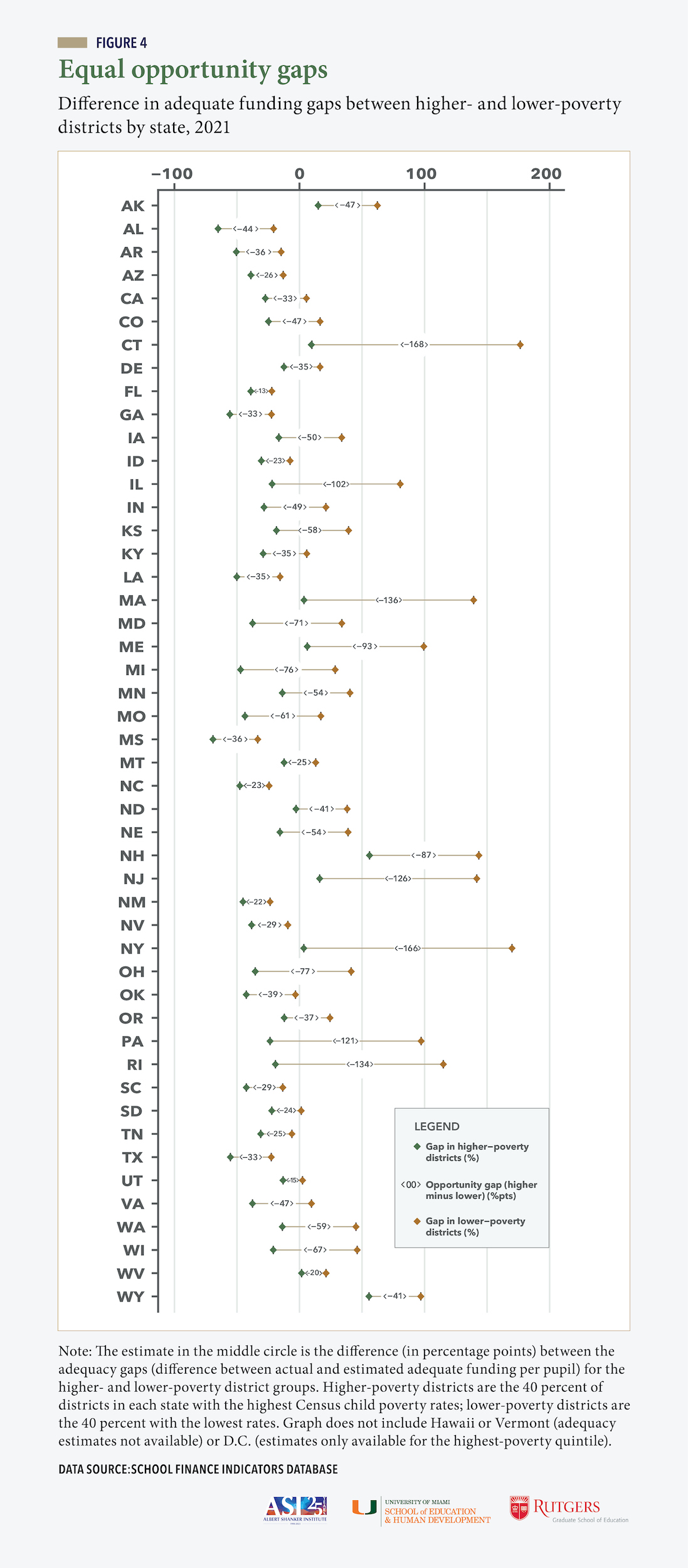
The gaps are presented, by state, in Figure 4.[8] For example, in Alaska, the highest-poverty districts (teal diamond) spend about 15 percent above estimated adequate levels, and the lowest-poverty districts (orange diamond) spend about 62 percent above adequate levels. The “opportunity gap” is therefore 15 minus 62 = -47 percentage points (reported in the line between the diamonds). Note that it doesn’t matter whether the two diamonds are above or below adequate; what matters is the “space” between them. As discussed above, equal opportunity and statewide adequacy as we define them are independent measures.
Figure 4 makes it very clear that unequal opportunity is universal in the U.S. In all states, higher-poverty districts are funded less adequately than lower-poverty districts (the teal diamonds are to the left of the orange diamonds). But, again, we are particularly interested in comparing states, and so variation in the magnitude of these gaps is our primary focus.
We find extremely large opportunity gaps in Connecticut (-168 percentage points), New York (-166), Massachusetts (-136), Rhode Island (-134), and New Jersey (-126). These are all northeastern states with relatively high statewide adequacy overall (see Figure 3) but extensive income and wealth inequality. To be clear, many higher-poverty districts in these states, like higher-poverty districts throughout the nation, are poorly funded relative to costs, which drives down adequacy for these districts (the teal diamonds in Figure 4). But the opportunity gaps are very much exacerbated at the lower-poverty end of the spectrum (orange diamonds). Affluent districts in these states tend to contribute massive amounts of local property tax revenue to their schools, thus widening the gaps in adequacy between higher- and lower-poverty districts. In other words, in these states, large opportunity gaps are often due as much to the highly adequate funding in affluent districts as they are to the inadequate funding in poorer districts. From this perspective, some degree of unequal opportunity (as we define it) may be inevitable, as we would never suggest that these wealthier districts should decrease their local investment in their schools. We do argue, however, that states can and should “raise the floor” for higher-poverty districts and narrow these gaps with targeted state aid. We’ll return to this in the recommendation section, below.
Conversely, the opportunity gaps are relatively small in Florida (-13 percentage points), Utah (-15), West Virginia (-20), New Mexico (-22), Idaho (-23), and North Carolina (-23). In most of these states, funding is widely inadequate overall, and it is too low to generate substantial inequality. Put differently, educational opportunity, though unequal in absolute terms, is more equal in these states in no small part because most districts get very little funding (relative to estimated costs).
.
A quick look at equal opportunity and progressivity
.
School funding is said to be “progressive” when higher-poverty districts receive (or spend) more than lower-poverty districts. If, in contrast, higher-poverty districts receive (or spend) less, then we would call this “regressive” funding. Since costs (i.e., adequate funding levels) tend to increase with poverty, progressivity is a necessary feature for achieving equal opportunity (and adequacy as well), and progressivity measures are a common and useful tool for assessing states’ finance systems. When evaluating states’ systems, however, the better question is whether spending is progressive enough—that is, whether funding increases with poverty at the same rate as do costs. This is what our opportunity gaps are designed to measure.
We illustrate this relationship in Table 1, which compares national averages for a few funding and contextual measures between lower-poverty districts (the 40 percent lowest-poverty districts in each state) and higher-poverty districts (the 40 percent of districts in each state with the lowest poverty rates).
As is the case with virtually all finance measures, the progressivity of K-12 spending (and revenue) varies widely by state, as do all the other measures presented in Table 1. But for the purposes of this quick illustration, we will just view national averages. Bear in mind that the actual dollar amounts here (in rows A and B) are less important than the difference between them (presented in the rightmost column); these gaps would not change appreciably were we to increase or decrease our benchmark student outcome goal (national average math and reading scores in grades 3-8). Also note that district poverty quintiles are defined state-by-state, and so the estimates below are just a rough approximation of the national differences in spending and costs by district poverty.
In row A of Table 1, we can see that actual unadjusted total spending is progressive.[9] Higher-poverty districts spend roughly 21 (20.8) percent more than lower-poverty districts. This is due in part to federal aid, which constitutes only about 10 percent of all K-12 funding but is distributed in a highly progressive fashion.
However, Table 1 also shows that estimated adequate funding (row B) increases with poverty far more quickly, with our cost targets, on average, coming in roughly 90 (89.0) percent higher for higher-poverty districts compared with their lower-poverty counterparts. As a result, the national average opportunity gap (row C, rightmost column) is approximately -40 percentage points. In other words, unadjusted spending is progressive, but not sufficiently progressive to meet the rise in estimated costs.
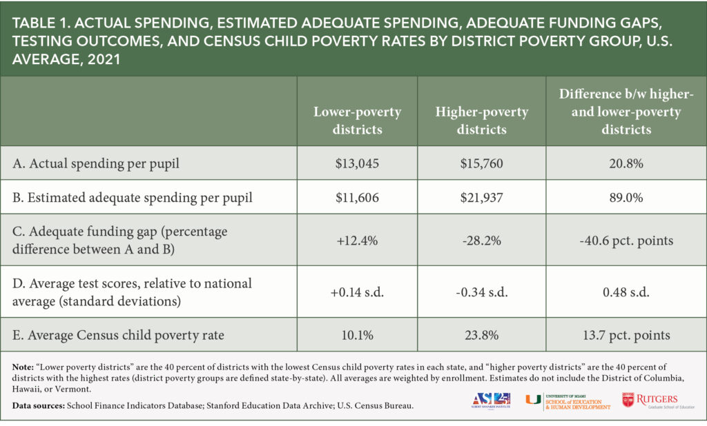
This gap in estimated costs—the idea that funding should be roughly twice as high (90 percent higher) in higher-poverty compared with lower-poverty districts—might seem surprisingly large. To contextualize this illustrative estimate, we also compare two additional statistics in Table 1. First, in row D, we present the average testing outcomes for both groups, measured in terms of the difference between these students and the national average (in standard deviations). Students in higher-poverty districts, on average, score roughly 0.34 standard deviations (s.d.) below the national average, while their peers in lower-poverty districts score about 0.14 s.d. above the national average. This is roughly equivalent to a 20 percentile increase. Making up such a large gap would require a commensurately large increase in resources.
Moreover, in row E, we see a similar difference in Census child poverty rates, with higher-poverty districts serving populations with poverty rates that are, on average, almost 25 (23.8) percent, compared with about 10 (10.1) percent in lower-poverty districts. We would, of course, expect that poverty is higher in higher-poverty districts, but this is a very large discrepancy, and it has a considerable impact on costs. Higher-poverty districts face challenges, such as trouble recruiting and retaining teachers, making it even harder for them to make up the gaps in student outcomes shown in row D (Hanushek, Kain, and Rivkin 2004; Lankford, Loeb, and Wyckoff 2002).
We cannot say whether 90 percent is the “correct” national difference in costs between higher- and lower-poverty districts. But we would suggest that it is well within realistic limits, given the gaps in student outcomes and poverty rates between these groups and the hurdles they must overcome to close those gaps. It is also consistent with the literature on the impact of additional spending on testing outcomes (Jackson and Mackevicius 2023). Frankly, even if the “correct” gap in adequate spending between higher- and lower-poverty districts is half as large as suggested in Table 1, it would still be more than double that in actual spending (21 percent).
In any case, the larger point here is that progressivity matters, but by itself it is not enough for an evaluation of states’ K-12 funding systems. Different states require different degrees of progressivity (in some states, the gap in costs is well above 90 percent, and in other states it is well below), and it is very difficult to adjudicate whether funding is progressive enough without cost estimates.
Equal opportunity by student race and ethnicity
Given the well-documented association between income/poverty and race and ethnicity, it is not entirely surprising that we should find gaps in K-12 funding adequacy by student race and ethnicity. That is, if students of color are overrepresented in lower-income districts, and lower-income districts tend to be less adequately funded than higher-income districts, then students of color will be more likely to attend schools in districts with below-adequate funding.
It is nonetheless important to examine these discrepancies, as doing so illustrates the multidimensionality of unequal educational opportunity in the United States, as well as the intersection of school funding and racial/ethnic segregation, both present and past (Baker, Di Carlo, and Green 2022). In addition, there is evidence that these race-/ethnicity-based funding gaps cannot be “explained away” by poverty (Baker et al. 2020).
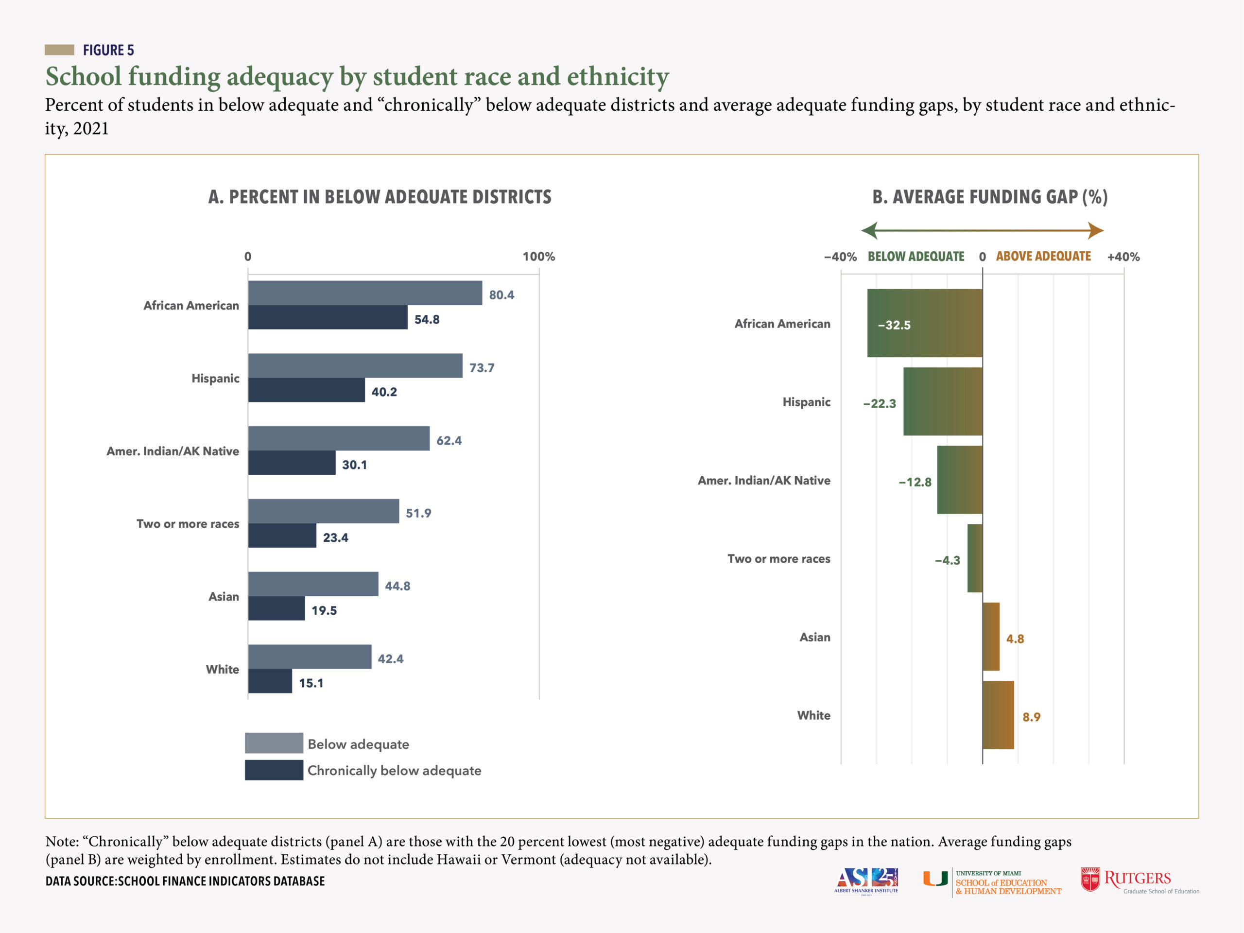
In panel A of Figure 5, we present the percent of students across all states attending districts with funding below estimated adequate levels and the percentage in chronically below adequate districts in 2021, by student race and ethnicity.
We find that 42 percent of white students attend districts with negative gaps, compared with 80 percent of African American students and 74 percent of Hispanic students.[10] In other words, African American students are about twice as likely as their white peers to attend school in a district with below-adequate funding, while Hispanic students are about 75 percent more likely to do so. Similarly, African American students are over 3.5 times more likely than white students to attend chronically underfunded districts (55 versus 15 percent, respectively), while Hispanic students are over 150 percent more likely (40 versus 15 percent).
We also find comparably large discrepancies when such gaps are defined in terms of adequate funding gaps (panel B of Figure 5). For example, the typical African American student’s district spends almost 33 percent below estimated adequate levels, whereas the typical white student’s district spends about 9 percent above our cost targets (for an opportunity gap of over -40 points). To view the results for individual states (funding gaps only), see Appendix Table A3.
These race- and ethnicity-based discrepancies in funding adequacy, like those based on district poverty, reflect the failure of most states to provide equal educational opportunity for their students, regardless of their backgrounds or circumstances. And this is particularly salient given that not a single state includes race and ethnicity as a factor in the allocation of K-12 revenue.
OVERALL STATE SCORES
The complexity and multidimensionality of school finance systems belie simple characterization, and assessing systems is extremely difficult, even when you focus on a small group of measures. In fact, as is evident throughout this report, it is most useful to interpret the results of one measure while referring to the others. For instance, when evaluating statewide adequacy, we have referred to states’ fiscal effort levels to assess the degree to which they have the capacity to increase funding on their own.
This suggests that boiling states’ systems down to single scores or ratings is necessarily reductive and risks oversimplification. On the other hand, we acknowledge that summative ratings, interpreted properly, can be useful. In Table 2, we present simple characterizations of effort, statewide adequacy, and equal opportunity in all states, with designations of high, medium, or low defined as the top, middle, and bottom one-third of states on each measure.
We also present an overall score (and rank) for each state. These overall scores are calculated very simply using our three core indicators. They are a weighted average of the following five components (each component is normalized, and the weights are in parentheses):[11]
Statewide adequacy (weight: 60 percent);
- Percent of students in districts with above adequate and not chronically below adequate funding (30 percent);
- Adequate funding gap, or percent difference between actual and required spending (30 percent);
Fiscal effort (30 percent);
- GSP-based (15 percent);
- API-based (15 percent);
Equal opportunity: difference in adequate funding gap between highest- and lowest-poverty districts (10 percent);
A couple of caveats are in order. First, each state’s overall score, as well as its rating on our three core indicators, represents its performance relative to other states, and not to any absolute standard of “good” or “bad.” In other words, states with higher scores do not necessarily have good systems per se, only better systems compared with other states on our selected measures using our selected weights. And the same point applies to the “high, medium, low” ratings for each of our three core indicators in Table 2. For instance, if a state has a rating of “high” on our equal opportunity measure, this does not necessarily mean that state exhibits highly equal opportunity by any absolute standard (as shown in Figure 4, no state achieves this). It only means that its equal opportunity score is among the top third in the nation. Second, and most obvious, the measures we have selected, as well as the weights we have assigned, reflect our subjective judgments as to the importance of each indicator.
In Table 2, an overall score of 50 can be roughly interpreted as average. Ranks may reflect differences in unrounded scores. Scores are not available for the District of Columbia, Hawaii, and Vermont because they are missing one or more of the measures used to calculate the scores.
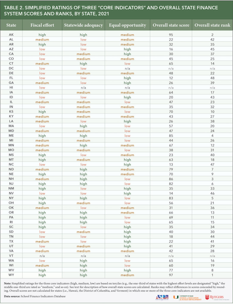
There are no surprises in Table 2. Wyoming and Alaska, with their high effort and widely adequate funding coupled with only moderately unequal opportunity, top the list with scores of 97 and 95, followed somewhat distantly by New Hampshire (86), Maine (85), New York (83), and New Jersey (82).
Conversely, Florida (12), North Carolina (13), Nevada (14), Arizona (16), and Tennessee (18) receive the lowest scores. These lowest-scoring states are still considerably above the hypothetical minimum score (1) because none of them is bottom of the pack on all three measures. Florida, for example, has among the nation’s lowest effort levels and statewide adequacy scores, but its equal opportunity score is the best in the nation, with an opportunity gap of “only” -13 percentage points.
Several of the states that perform well on our measures happen to generate substantial revenue through the extraction of natural resources (e.g., via severance taxes). This includes our top two highest scoring states of Wyoming and Alaska, as well as two other states in the top 10 (North Dakota and West Virginia). This is a particularly volatile source of revenue (e.g., due to changes in energy prices), and education funding in these states can therefore fluctuate quite dramatically over relatively short periods of time, but this revenue certainly contributes to these states’ relative performance on our measures.
POLICY RECOMMENDATIONS
The enormous “under the hood” heterogeneity of state school finance systems means that any attempt to offer national recommendations will inevitably be more general than specific. States’ systems are complex, develop over time, and reflect many years of political compromises. The end goal here is universal—all districts, and therefore all students, should have what they need to achieve common (and hopefully desirable) outcomes—but the specific reforms that can help accomplish that goal will always vary state by state.
That said, there are general principles that apply across all states, and these principles lend themselves naturally to sensible policy recommendations.
Better targeting of funding (especially state aid). The backbone of any state finance system is the procedure by which target funding levels are determined for each district. Virtually all states set these targets, whether explicitly or implicitly. If they not determined properly and rigorously, funding may appear adequate and equitable when it is not, and policymakers may not even realize it. Ideally, these targets should represent reasonable calculations of how much funding each district needs to achieve the common student outcome goal(s) chosen by the state, given its student population and other contextual factors (e.g., labor costs).
- Audit and reform formulas/targets. Although we would suggest using state-specific, output-based cost models to set these targets, there are alternative approaches that might also be feasible (Baker 2018). In any case, as a first step, all states should routinely “audit” their funding targets or levels by comparing them with estimates from analyses using multiple approaches that account for student and district characteristics that influence costs (e.g., Atchison et al. 2020; Kolbe et al. 2019; Taylor et al. 2018). States should then adjust their formulas based on the results, with the goal being to drive additional state aid to districts based on their need (targets) and capacity to produce local revenue.
- Eliminate regressive “stealth” policies. District funding targets, and thus the equity-producing benefits of state aid, are also compromised by policies in many states that are often buried in complex legislation or overlapping formulas that can require in-depth analysis to uncover. For instance, several states have enacted provisions by which districts are entitled to some minimum level of state aid regardless of their needs or local capacity, whereas others provide local tax relief in the form of additional state aid. Similarly, states often maintain multiple state revenue streams on top of their general formulas, including, for example, flat-rate block grants that are also distributed without reference to costs or local wealth (Baker and Corcoran 2012). States should thoroughly review their systems, identify these policies, and remove them. Any state aid that is not allocated according to need and local capacity will tend to exacerbate unequal opportunity, while also failing to maximize the adequacy benefits of state revenue.
Increase funding to meet student needs where such funding is inadequate. This is, perhaps, the most obvious of our recommendations, but we would emphasize that the point here is not simply to increase funding. It is, once again, to ensure that funding is commensurate with costs/need, with a particular focus on allocating enough state aid to compensate for variation in local capacity. Our adequacy estimates are designed to assess statewide adequacy and equal opportunity in each state relative to other states, but in reality, all states set their own outcome goals, and so the total amount of funding required can vary accordingly, even between states with similar student populations, labor costs, etc. In general, however, for effective targeting of funding to achieve adequacy and equal opportunity, there must be enough funding.
- Increase local revenue contributions where need and capacity are high. In states where funding is widely inadequate relative to costs, this might include a substantial increase in local revenue from districts where capacity is sufficient but revenue is lower than would be expected from that capacity (Baker, Di Carlo, and Weber 2022). “Fair share” contributions of local revenue by districts are a stable foundation of good finance systems, and cracks in that foundation will compromise the benefits of state aid.
- Increase state aid in amounts commensurate with funding gaps. In most states, particularly those in which effort is medium or low (i.e., where there is capacity to raise more revenue), the key is increasing state revenue (e.g., from state sales and income taxes). State K-12 aid is the great equalizer in school finance systems, as it is typically distributed based on district need/capacity. In some states, adequate and equitable funding might require only a relatively modest increase in state aid and/or better targeting. In other states, larger increases are needed. This additional revenue might come from state tax increases and/or from promising possibilities for expanding state tax bases, such as state taxation on nonresidential property (Baker, Di Carlo, and Oberfield 2023; Brent 1999; Ladd 1976).
- Eliminate policies that constrain revenue growth. In some states, meaningful increases in resources may require the phasing out of policies that constrain revenue or spending growth (e.g., Colorado’s TABOR or Proposition 13 in California).
- Balance revenue “portfolios”: Finally, states should also examine their revenue “portfolios”—i.e., the composition of their revenue by source (state vs. local) and tax type (sales, income, property)—and consider making adjustments to maximize equity and minimize volatility during economic downturns; the latter tends to cause disproportionate harm in higher-poverty districts (Baker et al. 2023).
Distribute federal K-12 aid based on both need and effort/capacity. As we’ve shown in this report, the unfortunate truth is that many states with widely inadequate funding have the economic capacity to rectify that problem partially or even wholly by devoting a reasonable share of their economies to their schools. Several other states, in contrast, do put forth strong effort but their costs are so high (e.g., high-poverty student populations) and/or their economies are so small that they are essentially unable meet their students’ needs. For these latter states, additional federal education aid can serve as a vital bridge to more adequate and equitable funding.
- Supplemental federal “foundation aid”. We recommend some type of federal “foundation aid” approach, in which supplemental federal funds are targeted at districts with below-adequate funding in states that: 1) are already paying their “fair shares” in state and local revenue (as a proportion of their capacity); or 2) make progress toward achieving this reasonable minimum state and local effort level.
- We have shown elsewhere that such an approach, thanks to recent advances in data availability and modeling, is now a real possibility (Baker, Di Carlo, and Weber 2022).
- This kind of federal program, while admittedly ambitious, would not only ensure that federal aid is targeted at states and districts where it is most needed, but might also provide some incentive for states to boost their own effort levels, which, as we’ve shown, are at their lowest levels in decades.
Enhance federal monitoring of school funding adequacy, equity, and efficiency, and mandate more comprehensive K-12 finance data collection. The federal government has long played a productive role in collecting and disseminating education data. The data we use to evaluate state systems in the SFID is mostly collected by the federal government, and the U.S. Department of Education has quite robust analytical capabilities.
- Increase federal monitoring and guidance. We recommend that the Department of Education establish a national effort to analyze the adequacy and equity of states’ systems and provide guidance to states as to how they might improve their systems.
- This would include estimation and publication of measures such as wage adjustment indices and compilations of nationally normed outcome measures such as those published by the Stanford Education Data Archive, annual estimates of costs such as those of the NECM, and periodic (e.g., five-year) evaluation of adequacy and equity in states’ finance systems.
- It should also include evaluations of the overall efficiency of state and local spending (using NECM-style cost models), as well as of specific policies and practices on which new revenue might be spent.
- Require finance data reporting from nongovernmental entities that operate public schools Finally, the annual collection of local education agency finance data (the F-33 survey), which is carried out by the U.S. Census Bureau and published by the National Center for Education Statistics, should include public schools run by independent nongovernment organizations (most notably charter schools).
Although several of our recommendations focus on the federal role in K-12 funding, and federal funds can (and do) help, the bulk of the improvement in U.S. school funding policy will have to come from action on the part of states, as they are responsible for raising and distributing the vast majority of K-12 funds in the country. And these are essentially 51 different systems. They are all complex, and often difficult to understand for policymakers, parents, and the public. None is perfect, and virtually all have at least some redeeming features. Such complexity can be daunting and frustrating, but it has also allowed researchers over the decades to examine how variation in the design of systems leads to variation in results. The upside is that we generally know what a good finance system looks like. But evaluating and ultimately improving states’ systems starts with credible, high-quality data and analysis.
Based on our extensive experience collecting, analyzing, and disseminating finance data, and in collaboration with other researchers and organizations, we have designed and presented above a range of indicators that we believe capture the complexity of school finance in a manner that is useful and comprehensible to all stakeholders.
We are once again making all of our data and full documentation freely available to the public at the SFID website (https://schoolfinancedata.org), along with single-page profiles of each state’s finance system, online data visualizations, and other resources. It is our ongoing hope and intention that the SFID, including the data presented in this report, can inform our national discourse about education funding, as well as guide legislators in strengthening their states’ systems.
CORRECTION: The original version of this report included mislabeled rows in Appendix Tables A2 and A3. The full state names in the two tables were replaced with two-letter state abbreviations in the report, but the rows were not properly ordered to reflect the differences in alphabetical order between full state names and abbreviations, resulting in mismatches between abbreviations and estimates in several states. This has been corrected, and we apologize for the mistake.
Endnotes
References
Atchison, Drew, Jesse Levin, Bruce Baker, and Tammy Kolbe. 2020. Equity and Adequacy of New Hampshire School Funding: A Cost Modeling Approach. Washington, D.C.: American Institutes for Research.
Baker, Bruce D. 2017. How Money Matters for Schools. Palo Alto, CA: Learning Policy Institute.
Baker, Bruce D. 2018. Educational Inequality and School Finance: Why Money Matters for America’s Students. Cambridge, MA: Harvard University Press.
Baker, Bruce D. 2021. School Finance and Education Equity: Lessons from Kansas. Cambridge, MA: Harvard University Press.
Baker, Bruce D. 2023. School Funding in Missouri. Jefferson City, MO: Missouri Department of Elementary and Secondary Education.
Baker, Bruce D., and Matthew Di Carlo. 2020. The Coronavirus Pandemic and K-12 Education Funding. Washington, D.C.: Albert Shanker Institute.
Baker, Bruce D., Matthew Di Carlo, and Preston C. Green. 2022. Segregation and School Funding: How Housing Discrimination Reproduces Unequal Opportunity. Washington, D.C.: Albert Shanker Institute.
Baker, Bruce D., Matthew Di Carlo, and Zachary W. Oberfield. 2023. The Source Code: Revenue Composition and the Adequacy, Equity, and Stability of K-12 School Spending. Washington, D.C.: Albert Shanker Institute.
Baker, Bruce D., Matthew Di Carlo, and Mark Weber. 2022. Ensuring Adequate Education Funding For All: A New Federal Foundation Aid Formula. Washington, D.C.: Albert Shanker Institute.
Baker, Bruce D., and Sean P. Corcoran. 2012. The Stealth Inequalities of School Funding: How State and Local School Finance Systems Perpetuate Inequitable Student Spending. Washington, D.C.: Center for American Progress.
Baker, Bruce D., Ajay Srikanth, Robert Cotto, and Preston C. Green. 2020. “School Funding Disparities and the Plight of Latinx Children.” Education Policy Analysis Archives 28(135):1–26.
Baker, Bruce D., Mark Weber, and Ajay Srikanth. 2021. “Informing Federal School Finance Policy with Empirical Evidence.” Journal of Education Finance 47(1):1–25.
Brent, Brian O. 1999. “An Analysis of the Influence of Regional Nonresidential Expanded Tax Base Approaches to School Finance on Measures of Student and Taxpayer Equity.” Journal of Education Finance 24(3):353–78.
Bureau of Economic Analysis. 2023. Regional Data: GDP and Personal Income (Dataset). Washington, D.C.: Bureau of Economic Analysis.
Candelaria, Christopher A., and Kenneth A. Shores. 2019. “Court-Ordered Finance Reforms in the Adequacy Era: Heterogeneous Causal Effects and Sensitivity.” Education Finance and Policy 14(1):31–60.
Cornman, Stephen Q., Laura C. Nixon, Matthew J. Spence, Lori L. Taylor, and Douglas E. Geverdt. 2019. Education Demographic and Geographic Estimates (EDGE) Program American Community Survey Comparable Wage Index for Teachers (ACS-CWIFT) (NCES 2018-130). Washington, D.C.: National Center for Education Statistics.
Downes, Thomas. 2004. Operationalizing the Concept of Adequacy for New York State. Unpublished manscript.
Duncombe, William D., and John Yinger. 2007. “Measurement of Cost Differentials.” Pp. 257–75 in Handbook of Research in Education Finance and Policy, edited by H. F. Ladd and E. B. Fisk. Mahwah, N.J.: Lawrence Erlbaum Associates, Inc.
Duncombe, William, and John Yinger. 1997. “Why Is It So Hard to Help Central City Schools?” Journal of Policy Analysis and Management 16(1):85–113.
Duncombe, William, and John Yinger. 1998. “School Finance Reform: Aid Formulas and Equity Objectives.” National Tax Journal51(2):239–62.
Duncombe, William, and John Yinger. 1999. “Performance Standards and Educational Cost Indexes: You Can’t Have One Without the Other.” Pp. 260–97 in Equity and Adequacy in Education Finance: Issues and Perspectives, edited by H. F. Ladd, R. Chalk, and J. S. Hansen. Washington, D.C.: National Academy Press.
Duncombe, William, and John Yinger. 2000. “Financing Higher Student Performance Standards: The Case of New York State.” Economics of Education Review 19(4):363–86.
Duncombe, William, and John Yinger. 2005. “How Much More Does a Disadvantaged Student Cost?” Economics of Education Review 24(5):513–32.
Figlio, David N., and Maurice E. Lucas. 2004. “What’s in a Grade? School Report Cards and the Housing Market.” American Economic Review 94(3):591–604.
Geverdt, Doug. 2018. Education Demographic and Geographic Estimates Program (EDGE): School Neighborhood Poverty Estimates – Documentation (NCES 2018-027). Washington, D.C.: National Center for Education Statistics.
Handel, Danielle Victoria, and Eric A. Hanushek. 2023. “U.S. School Finance: Resources and Outcomes.” in Handbook of the Economics of Education, edited by S. J. Machin, L. Woessmann, and E. A. Hanushek. Amsterdam: Elsevier.
Hanushek, Eric A., John F. Kain, and Steven G. Rivkin. 2004. “Why Public Schools Lose Teachers.” The Journal of Human Resources 39(2):326–54.
Imazeki, Jennifer, and Andrew Reschovsky. 2004. “Is No Child Left Behind an Un (or Under) Funded Federal Mandate? Evidence from Texas.” National Tax Journal 57(3):571–88.
Jackson, C. Kirabo. 2020. “Does School Spending Matter? The New Literature on an Old Question.” Pp. 165–86 in Confronting Inequality: How Policies and Practices Shape Children’s Opportunities, edited by L. Tach, R. Dunifon, and D. L. Miller. Cambridge, MA: National Bureau of Economic Research.
Jackson, C. Kirabo, Rucker C. Johnson, and Claudia Persico. 2016. “The Effects of School Spending on Educational and Economic Outcomes: Evidence from School Finance Reforms *.” The Quarterly Journal of Economics 131(1):157–218.
Jackson, C. Kirabo, and Claire Mackevicius. 2023. “What Impacts Can We Expect from School Spending Policy? Evidence from Evaluations in the U.S.” American Economic Journal: Applied Economics2.
Jackson, C. Kirabo, Cora Wigger, and Heyu Xiong. 2021. “Do School Spending Cuts Matter? Evidence from the Great Recession.” American Economic Journal: Economic Policy 13(2):304–35.
JLARC, Virginia. 2023. Virginia’s K-12 Funding Formula. Richmond, VA: Joint Legislative Audit and Review Commission (JLARC), General Assembly of the Commonwealth of Virginia.
Kolbe, Tammy, Bruce Baker, Drew Atchison, and Jesse Levin. 2019. Pupil Weighting Factors Report (Act 173 of 2018, Sec. 11). Montpelier, VT: Vermont Agency of Education.
Kolbe, Tammy, Bruce D. Baker, Drew Atchison, and Jesse Levin. 2019. Pupil Weighting Factors Report: Report to the House and Senate Committees on Education, the House Committee on Ways and Means, and the Senate Committee on Finance. Montpelier, VT: State of Vermont, House and Senate Committees on Education.
Ladd, Helen F. 1976. “State-Wide Taxation of Commercial and Industrial Property for Education.” National Tax Journal 29(2):143–53.
Lafortune, Julien, Jesse Rothstein, and Diane Whitmore Schanzenbach. 2018. “School Finance Reform and the Distribution of Student Achievement.” American Economic Journal: Applied Economics 10(2):1–26.
Lankford, Hamilton, Susanna Loeb, and James Wyckoff. 2002. “Teacher Sorting and the Plight of Urban Schools: A Descriptive Analysis.” Educational Evaluation and Policy Analysis 24(1):37–62.
Leachman, Michael, Kathleen Masterson, and Eric Figueroa. 2017. A Punishing Decade for School Funding. Washington, D.C.: Center on Budget and Policy Priorities.
National Center for Education Statistics. 2022. National Assessment of Educational Progress (NAEP), 2020 and 2022 Long-Term Trend (LTT) Reading and Mathematics Assessments. Washington, D.C.: U.S. Department of Education, Institute of Education Sciences, National Center for Education Statistics.
National Center for Education Statistics. 2023a. Common Core of Data: Local Education Agency (School District) Finance Survey (F-33) (Dataset). Washington, D.C.: National Center for Education Statistics.
National Center for Education Statistics. 2023b. Common Core of Data: Public Elementary/Secondary School Universe Survey (Dataset). Washington, D.C.: National Center for Education Statistics.
Nguyen-Hoang, Phuong, and John Yinger. 2011. “The Capitalization of School Quality into House Values: A Review.” Journal of Housing Economics 20(1):30–48.
Reardon, Sean F., Andrew D. Ho, Benjamin R. Shear, Erin M. Fahle, Demetra Kalogrides, Heewon Jang, and Belen Chavez. 2021. Stanford Education Data Archive (Version 4.1). Palo Alto, CA: Stanford University.
Taylor, Lori L. 2014. Extending the NCES Comparable Wage Index. College Station, TX: Texas A&M University.
Taylor, Lori L., William J. Fowler, and Mark Schneider. 2006. A Comparable Wage Approach to Geographic Cost Adjustment (NCES 2006-321). Washington, D.C.
Taylor, Lori, Jason Willis, Alex Berg-Jacobson, Karina Jaquet, and Ruthie Caparas. 2018. Estimating the Costs Associated with Reaching Student Achievement Expectations for Kansas Public Education Students: A Cost Function Approach. San Francisco, CA: WestEd.
U.S. Census Bureau. 2023a. Annual Survey of School System Finances: Public Elementary-Secondary Education Finance Data (Dataset). Washington, D.C.: U.S. Census Bureau.
U.S. Census Bureau. 2023b. National and State Population Estimates (Dataset). Washington, D.C.: U.S. Department of Commerce, Bureau of the Census.
U.S. Census Bureau. 2023c. Small Area Income and Poverty Estimates (1993-2022) [Dataset]. Washington, D.C.: U.S. Census Bureau.
Appendix tables
Download the full report to view appendix tables.
APPENDIX TABLE A1. Information on data sources
APPENDIX TABLE A2. Statewide adequacy estimates by state, 2021
APPENDIX TABLE A3. Adequate funding gaps by district poverty and student race and ethnicity, by state, 2021
Authors: Bruce D. Baker; Matthew Di Carlo; Mark Weber
Download full report (PDF)
View one-page state finance system profiles
Download full dataset
Use online data visualizations
Latest News
 UPDATED ANNUAL REPORT, PROFILES, AND DATASETS AVAILABLE
February 2026: Read the eighth edition of our annual report, view your state’s one-page finance profile, use our data visualizations, or download the full state-level dataset.
Latest Annual Report
 The Adequacy and Fairness of State School Finance Systems (8th edition)
The eighth edition of our annual report presenting findings on effort, statewide adequacy, and equal opportunity in state school finance systems. Published February 2026.
Latest Research Briefs
 State School Finance System Profiles (2022-23 school year)
One-page profiles summarizing the key results on effort, statewide adequacy, and equal opportunity for all 50 states and D.C. View your state’s profile. Published February 2026.


Copyright © 2022-2023 Albert Shanker Institute | All Rights Reserved